I am reading a paper to learn about the theory of Radiance,. A Ray Tracing Solution for Diffuse Interreflection, but there are some things I don’t understand, so I would like to know two things.
①
In Equation 2, the upper limit of sigma addition is n, 2n. Why is this? If we think of it as a transformation from Equation 1 to Equation 2, wouldn’t it be n, 4n?
②
I have derived the inequality in equation (3a) using the first order Taylor expansion, how can this be derived?
I tried to prove that this inequality holds from Taylor’s theorem, but I could not derive it.
If you don’t mind, I’d like to know the process of deriving the equation.
I think the 2n2 in equation 2 is just the number of samples… I see it as a Montecarlo integration, we are calculating the average of a bunch of samples. If you see the Sums, you have 1..n and 1..2n; meaning n*2n = 2n2 samples. These samples are distributed in the hemisphere. In the Rendering with Radiance book that equation is different, I think, as it does not assume n an 2n samples; but n and m; and m*n = ambient_divitions
I have not studied Equation 3 at all…
PS: I am afraid Greg will destroy this answer, but I hope you find it useful for a couple of minutes before that.
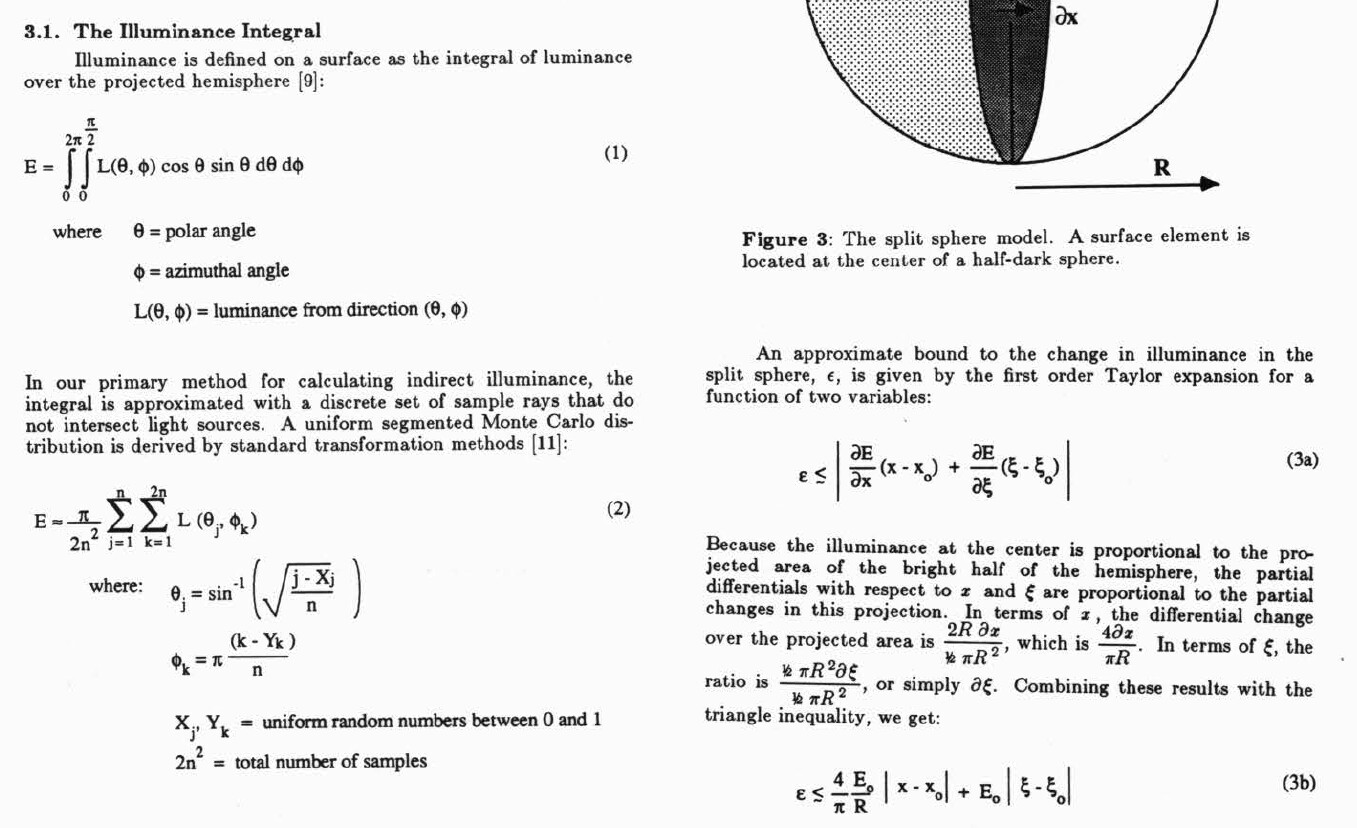
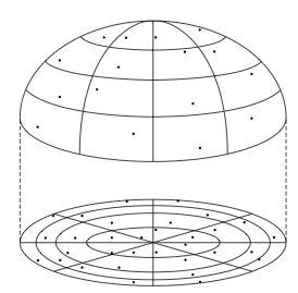
Not to destroy anything, but at some point, there is no need to discuss the details of the 1988 paper. We can actually divide phi and theta however we like in the sum – we chose this as a reasonable compromise for the division cell aspect ratios, though it’s still pretty bad. (See Figure 12.7 from “Rendering with Radiance,” reproduced below.)
Likewise, we don’t use the split sphere estimate for calculation spacing anymore. We have supplanted this method in the current version with a more accurate Hessian calculation due to Schwarzhaupt, Wann Jensen and Jarosz:
They use the Shirley-Chiu hemisphere subdivision, which does a much better job and simplifies neighbor relationships. We also fixed an issue they had with locally shaded regions, as described in my 2014 workshop talk.
Eq. (3a) isn’t derived from Taylor’s expansion – it is the first-order Taylor’s expansion for any two-variate function. Eq. (3b) is the Taylor’s expansion for the split sphere condition, and is computed by differentiating the formula for projected area as a function of position and orientation from the test point.
As I said, none of this is currently used by Radiance, so is really only of historical interest.