Hi everyone,
I’ve been building a browser-based horticultural lighting simulation tool on top of Radiance and wanted to share the details here for feedback from people with more Radiance experience than I have. The tool compares three lighting system modes in a closed room CEA benchmark and is designed to make canopy uniformity comparisons easier to inspect.
The two things I’d most value scrutiny on are: (1) the photon-native solve pipeline and (2) the basis-matrix optimization approach for ring-wise power assignment — both described below. The source-model section is long but I’ve tried to be explicit about what is and isn’t claimed for each mode.
I’m happy to provide a link to the tool if the community is interested in messing around with it.
Source models
The three modes are not modeled the same way, and I want to be precise about the distinctions.
Modular LED surrogate (SMD mode)
A module-level physical surrogate — not a finished luminaire IES. Each module is a 150 mm × 150 mm PCB with a 120 mm × 120 mm emitting window carrying 145 LED sites in a fixed package mix: 52 warm-white, 52 cool-white, and 41 deep-red. The optical stack is modeled explicitly:
- PMMA lid: 128 mm × 128 mm × 3 mm, n = 1.49, target transmission ~0.92
- PTFE cavity liner: reflectance 0.97, thickness 0.508 mm, surrounding the emitting aperture
Electrical and optical baseline. At an estimated operating current of ~233 mA per string, nominal package electrical assumptions are 0.68 W for the white channels and 0.44 W for deep red. Per-channel PPE values are estimated at 2.73 µmol/J (warm-white), 2.81 µmol/J (cool-white), and 4.13 µmol/J (deep-red), giving a blended module base efficacy of ~3.00 µmol/J and a total PPF of ~269.6 µmol/s before optical cover and driver losses. After applying 92% PMMA transmission (without taking additional credit for PTFE photon recovery), estimated module output is ~248.0 µmol/s. With driver losses (HLG-185H-C700B or HLG-320H-C700B), estimated wall-plug efficacy is ~2.60–2.62 µmol/J.
Droop and thermal modeling. The engine computes continuous dynamic efficacy per module using component-level V-I (fC_vs_fV) and efficacy (ppe_vs_fC) characterization curves. The solver interpolates forward voltage and current for both the red and white channels at each driven current state, evaluating exact electrical power and relative PPE multiplier per channel. Non-system losses are applied as continuous multipliers: driver efficiency 0.96, wiring efficiency 0.99, and a continuous thermal derate coefficient scaled to module wattage to model junction temperature rise.
The engine applies a concentric ring-wise power assignment strategy (described in the layout and solver sections below) rather than a flat per-module wattage. No measured finished luminaire IES is claimed for this mode.
1000 W DE HPS surrogate
A physically parameterized surrogate for a broad distribution horticultural HPS fixture. Not presented as measured manufacturer photometry.
- Envelope: 22.2 in × 9.7 in × 7.8 in
- Lamp: horizontal double-ended arc-tube, approximated by an 8-face luminous prism
- Reflector: explicit wide-reflector geometry with shallow gull-wing side panels, top cover, and end plates; RGB reflectance 0.92 / 0.91 / 0.87; semi-specular 0.16; roughness 0.03
- Nominal output: 2050 µmol/s at 1050 W (~1.95 µmol/J)
Lamp-level source output is set slightly above fixture-level emitted output to absorb reflector losses. Layout is by nominal coverage footprint (4 ft × 4 ft or 5 ft × 5 ft grid) rather than exact envelope packing. Mounting height: 36 in.
Conventional LED (IES-composed mode)
This mode is different in kind from the two above. It constructs a 6-bar fixture by repeating a single bar-level IES source six times across an explicit fixture envelope. It is not a physically parameterized surrogate and does not claim a measured one-piece horticultural luminaire IES for the assembled fixture.
- Fixture envelope: 47.75 in × 43.44 in; bar envelope 47.75 in × 4.46 in × 1.56 in
- Bar center-to-center spacing: ~7.80 in
- IES archetype: bundled
conventional.ies, a 4 ft strip-light style photometric file reporting ~8159.6 lm and 46 W per bar - Lumens-to-photons conversion: 0.015 µmol/s per lumen (configurable scalar)
- ies2rad normalization: Radiance luminous-efficacy constant of 179 lm/W
- Fixture-level PPF target: 2200 µmol/s (~366.7 µmol/s per bar)
- PPE assumption for electrical reporting: ~2.7 µmol/J
This preserves directional bar-driven canopy structure and spacing sensitivity. The main modeling limitation is that the bar-level IES is a strip-light archetype rather than a measured source for this fixture class, and the lm → µmol/s conversion uses a single broadband scalar rather than a spectrally resolved model.
PPFD methodology — photon-native Radiance solve
Rather than running a standard lux solve and applying a post-hoc lm → µmol/s correction, the engine normalizes all emitters into µmol units before calling rtrace. Because emitters are authored with equal RGB values representing photon flux, the three returned channels from rtrace are treated as already being in photon units, and scalar PPFD is recovered by:
Source authoring differs by mode:
- SMD and HPS modes: light materials are written directly in µmol/s/sr/m² with equal RGB values.
- Conventional LED mode: IES lumens are converted to photons via the 0.015 µmol/s per lumen factor, then normalized through the 179 lm/W
ies2radconstant, so the scaled source is traced purely as a photon emitter.
The main approximation here is in the IES path: a single broadband scalar replaces a wavelength-resolved spectral model. I’d welcome feedback on whether this is an acceptable approximation for comparative canopy uniformity work, or whether it introduces a systematic error I should be treating differently.
Layout framework
Concentric ring placement
The modular LED system uses a concentric ring layout that serves two purposes: it determines both physical module placement and the control zone structure used by the optimization solver. The room footprint is mapped to an integer module grid of width N_x and height N_y after snapping physical dimensions to the module mechanical pitch (152.4 mm × 165.0 mm).
Square mode begins with a fixed X-pattern centerpiece of n_0 = 5 modules. For t concentric rings, each ring j contains r_j = 4j + 4 modules, giving a total module count of:
This recurrence is unbounded, enabling arbitrarily large square layouts while preserving the same ring-indexed control structure.
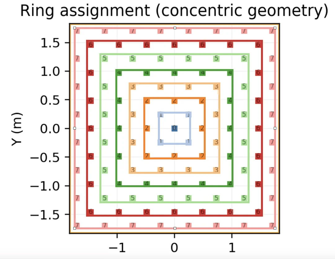
Rectangular extension handles non-square footprints (N_x \geq N_y) by building around a central linear base strip of length n modules. With t = (N_y - 1)/2 rings stacked above and below, ring j contains r_j = 2n + 4j - 2 modules, and the outermost row length sets the required base-strip length as n = N_x - N_y + 2. Total module count:
Tiling. When a target room exceeds the size of a single square cell, the generator tiles square cells and introduces a minimal rectangular extension only when required by the room aspect ratio, connected by a single centralized linear strip. Square sub-arrangements are preferred because square zoning produces more symmetric control behavior than rectangular extensions. The resulting module map is realized physically using a small family of fixture types (X-pattern, linear sections, corner sections) while preserving the generated placement and ring zoning structure.
All arrangements are centered inside the usable room span after the outer wall inset and mechanical footprint allowances.
Basis-matrix solver and optimization
The concentric-zone power assignment is determined by a Radiance-based linear superposition approach. Rather than re-rendering the full scene for every candidate weight combination, the solver first constructs a response basis from ring-isolated simulations.
Basis construction
For a layout with K concentric control rings sampled at n sensor locations, each ring is rendered in isolation at a defined unit drive level while all other rings are off. The resulting PPFD values across the sensor grid form a column vector. Collecting these columns yields a response matrix A \in \mathbb{R}^{n \times K}. For any ring-weight vector w \in \mathbb{R}^{K}, the predicted canopy-plane field is:
Once A has been generated for a given room geometry and layout, candidate ring weights can be evaluated rapidly without repeated full ray-trace calls.
Optimization formulation
The solver minimizes spatial deviation from a user-defined target mean PPFD \mu subject to control bounds and a mean-constraint:
subject to:
Here D is a first-difference matrix penalizing abrupt ring-to-ring transitions, and \lambda_s, \lambda_r are optional smoothness and ridge regularization coefficients. In the default workflow, the variance minimization term is dominant and regularization is used only as needed to suppress non-physical weight oscillation. Solutions that fail to satisfy the mean constraint within the specified tolerance are rejected.
The ring-wise power assignment produced by the solver feeds directly into the per-module efficacy and droop calculations described in the SMD source model section above.
Room model and benchmark setup
Simulations were run in a closed six-surface room: four walls, ceiling, and floor.
- Walls and ceiling: diffuse RGB 0.90 / 0.90 / 0.90, specularity 0.04, roughness 0.00 (intended to approximate panda film)
- Floor: diffuse reflectance 0.10 to reduce unrealistic floor-bounce uplift
- Canopy sensor plane: z = 0.005 m, physically adaptive rectangular grid, target sensor spacing 0.25 m with minimum grid counts enforced for smaller rooms
Mounting heights: 18 in for the SMD and conventional LED modes, 36 in for the DE HPS mode, reflecting typical deployment distances for each system class.
Convergence study (12 ft × 12 ft room, SMD mode)
I ran a three-preset convergence study targeting 1000 µmol/m²/s mean PPFD.
| Preset | -ab | -ad | -as | -aa | -ar | -dj | -ds | -dt | -dc | -dr | -lr | -lw |
|---|---|---|---|---|---|---|---|---|---|---|---|---|
| Standard | 3 | 512 | 128 | 0.22 | 48 | 0.35 | 0.40 | 0.08 | 0.50 | 1 | 6 | 2e-4 |
| Quality | 5 | 2048 | 512 | 0.12 | 96 | 0.65 | 0.20 | 0.03 | 0.85 | 3 | 12 | 5e-5 |
| Rigorous | 6 | 4096 | 1024 | 0.08 | 128 | 0.70 | 0.15 | 0.02 | 0.90 | 4 | 16 | 2e-5 |
PPFD uniformity metrics are essentially converged across all three presets (CV spread of ~0.22 percentage points). The more notable result is that Standard underreports required electrical input by roughly 10% relative to Quality and Rigorous — likely attributable to the lower -ab and -dc values and higher -ds accepting more direct sampling approximation. The precomputed bundles in the web application currently use the Standard preset, but based on this finding I may need to recompute the data bundles through the Quality preset.
| Preset | Watts in | Mean PPFD | Min PPFD | Max PPFD | CV | DOU |
|---|---|---|---|---|---|---|
| Standard | 4713.1 | 1000.00 | 946.66 | 1034.26 | 1.60% | 98.40% |
| Quality | 5228.7 | 1000.20 | 952.66 | 1036.79 | 1.47% | 98.53% |
| Rigorous | 5173.4 | 1000.32 | 952.41 | 1031.60 | 1.38% | 98.62% |
Questions for the community
- Does the photon-native solve approach look sound? Is the IES-path broadband scalar approximation a more significant methodological gap than I’m treating it as for comparative uniformity work?
- Do the convergence parameters and Quality preset selection look reasonable? Any settings I should be revisiting?
- Are the reflectance and room model assumptions fair for a closed room horticultural benchmark, or are there common pitfalls with this geometry worth guarding against?
- Is the source modeling distinction between the physically parameterized surrogates and the IES-composed mode described clearly and honestly enough, or does something read as overclaiming?
- Does the basis-matrix superposition approach — rendering each ring in isolation then combining — introduce any Radiance-specific issues I should be aware of? I’m relying on linear superposition holding at the zoning level given the predominantly diffuse room surfaces, but I’d welcome scrutiny on that assumption.
- Any other Radiance-specific pitfalls to watch for in a comparative workflow across geometrically and optically heterogeneous source models?
Since horticultural lighting is a less common Radiance use case, I’d especially appreciate feedback on any assumptions that look off.
Thanks for reading, and special thanks to Greg Ward / this community for creating such a brilliant tool.