Hello everyone,
I am trying to find a way to simulate annual spectral lighting. As far as I know, this has not been done so far, and the link related to the explanation of this method in frads is inactive.
Two approaches come to mind:
- Performing a point-in-time simulation for each hour considered (which is very time-consuming).
- Using a 2-phase or 2.5-phase method (as far as I know, BSDF files do not contain spectral information, so higher-phase methods cannot be considered for now).
Since EPW files do not contain spectral lighting data, we need to compute spectral lighting values based on the EPW file in both approaches.
First Method:
We can use the gensky command to read DHI and DNI values from the EPW file and generate the spectral lighting for each hour. Then, we can use the rtrace command and repeat this process in a loop for all the required hours.
I did this for two days (the summer solstice and the winter solstice) for a room with a window facing south, assuming a completely clear sky, and I encountered two issues:
- Throughout the night, the result is never zero, and there is always about 1 lux in the results.
- At sunrise and sunset, the light level increases dramatically, to the extent that during the winter solstice, it returned an infinite amount.
Summer solstice
| Column 1 | Column 2 | Column 3 | Column 4 | E | F | G | H | I | J | K | L | M | N | O | P | Q | R | S | T | U | V | W |
|---|---|---|---|---|---|---|---|---|---|---|---|---|---|---|---|---|---|---|---|---|---|---|
| hour | lux | mlux | 760 | 740 | 720 | 700 | 680 | 660 | 640 | 620 | 600 | 580 | 560 | 540 | 520 | 500 | 480 | 460 | 440 | 420 | 400 | 380 |
| 0 | 0.9819072 | 1.653156 | 0.004737538 | 0.00519847 | 0.005616502 | 0.005784307 | 0.005934488 | 0.005696022 | 0.004997215 | 0.004341822 | 0.003660811 | 0.003646896 | 0.003928697 | 0.00529061 | 0.006477665 | 0.008452562 | 0.01015819 | 0.01122887 | 0.01092604 | 0.008732359 | 0.007998057 | 0.003737103 |
| 1 | 0.9932547 | 1.680741 | 0.004791212 | 0.005260693 | 0.005683729 | 0.005849821 | 0.006002401 | 0.005774796 | 0.005055576 | 0.004404763 | 0.003704285 | 0.003698601 | 0.003981432 | 0.005364812 | 0.006578475 | 0.008584659 | 0.01032523 | 0.01142015 | 0.01112108 | 0.008898703 | 0.008160373 | 0.003827536 |
| 2 | 0.9747171 | 1.653589 | 0.004739539 | 0.005196732 | 0.005619172 | 0.005776088 | 0.005928566 | 0.005690116 | 0.004983216 | 0.00434636 | 0.003651197 | 0.003653235 | 0.003922968 | 0.00528499 | 0.006474639 | 0.00845163 | 0.01016595 | 0.01122902 | 0.01093276 | 0.008741657 | 0.008004189 | 0.003754346 |
| 3 | 0.9466258 | 1.599335 | 0.004537025 | 0.004982268 | 0.005388448 | 0.005541242 | 0.005685906 | 0.00545832 | 0.004783568 | 0.004166448 | 0.003509401 | 0.003511418 | 0.00377911 | 0.005087696 | 0.006233878 | 0.008156768 | 0.009821578 | 0.01087646 | 0.01060548 | 0.008498393 | 0.00780484 | 0.003669302 |
| 4 | 2.00E+28 | 1.37E+28 | 1.16E+26 | 9.86E+25 | 8.35E+25 | 6.87E+25 | 6.62E+25 | 6.75E+25 | 8.52E+25 | 9.79E+25 | 1.19E+26 | 1.34E+26 | 1.39E+26 | 1.27E+26 | 9.41E+25 | 8.27E+25 | 4.23E+25 | 6.44E+25 | 9.40E+25 | 9.56E+25 | 7.74E+25 | 2.75E+25 |
| 5 | 1.34E+30 | 6.68E+29 | 9.82E+28 | 9.43E+28 | 9.03E+28 | 8.37E+28 | 7.28E+28 | 6.29E+28 | 5.22E+28 | 4.54E+28 | 3.94E+28 | 3.74E+28 | 3.28E+28 | 2.90E+28 | 2.45E+28 | 2.00E+28 | 1.46E+28 | 9.45E+27 | 7.42E+27 | 3.65E+27 | 3.65E+27 | 1.29E+28 |
| 6 | 753.5671 | 872.1439 | 2.214651 | 2.413981 | 2.619195 | 2.802916 | 3.031773 | 3.244238 | 3.33143 | 3.496228 | 3.558532 | 3.746145 | 3.929284 | 4.294053 | 4.561444 | 4.799912 | 5.069962 | 5.218303 | 4.886383 | 3.821409 | 3.439213 | 1.553192 |
| 7 | 1146.103 | 1350.239 | 3.294459 | 3.571918 | 3.858605 | 4.123303 | 4.469591 | 4.808788 | 4.989076 | 5.324719 | 5.522193 | 5.869709 | 6.185718 | 6.668661 | 7.063069 | 7.391369 | 7.860149 | 8.225389 | 7.89331 | 6.375254 | 5.963206 | 2.813145 |
| 8 | 1483.009 | 1720.557 | 4.224508 | 4.566031 | 4.916071 | 5.247862 | 5.673632 | 6.103543 | 6.352626 | 6.813684 | 7.105041 | 7.560411 | 7.961694 | 8.507759 | 8.979553 | 9.355426 | 9.948486 | 10.47423 | 10.15281 | 8.329597 | 7.941362 | 3.836226 |
| 9 | 1874.271 | 2157.834 | 5.402536 | 5.829337 | 6.257264 | 6.672217 | 7.197861 | 7.737888 | 8.061912 | 8.652125 | 9.040513 | 9.617952 | 10.11722 | 10.75005 | 11.3075 | 11.71972 | 12.43922 | 13.10284 | 12.74011 | 10.51552 | 10.02701 | 4.848726 |
| 10 | 2484.493 | 2843.367 | 8.00515 | 8.567589 | 9.142307 | 9.67007 | 10.36147 | 11.06896 | 11.46656 | 12.24914 | 12.73883 | 13.45685 | 14.02347 | 14.69767 | 15.24939 | 15.58758 | 16.33002 | 17.05279 | 16.53347 | 13.66341 | 12.64225 | 5.907139 |
| 11 | 3366.708 | 3554.91 | 10.98722 | 11.71116 | 12.41887 | 13.08376 | 13.95263 | 14.8033 | 15.29774 | 16.25723 | 16.84599 | 17.68529 | 18.30643 | 18.98765 | 19.50505 | 19.6683 | 20.37017 | 21.08556 | 20.32775 | 16.77241 | 15.00163 | 6.708296 |
| 12 | 3668.293 | 3937.402 | 12.58924 | 13.39938 | 14.1717 | 14.91217 | 15.87919 | 16.81767 | 17.35386 | 18.40073 | 19.0492 | 19.96467 | 20.61212 | 21.28996 | 21.77701 | 21.87281 | 22.57344 | 23.27555 | 22.4259 | 18.50803 | 16.29683 | 7.13532 |
| 13 | 3526.006 | 3712.897 | 11.43809 | 12.18793 | 12.9184 | 13.62177 | 14.52067 | 15.40776 | 15.92367 | 16.91685 | 17.54213 | 18.43168 | 19.07926 | 19.79164 | 20.33553 | 20.51924 | 21.26141 | 22.03576 | 21.27967 | 17.59925 | 15.73381 | 7.038675 |
| 14 | 2763.081 | 3023.901 | 8.509103 | 9.108073 | 9.710766 | 10.27897 | 11.02461 | 11.77643 | 12.19055 | 13.01752 | 13.55343 | 14.31475 | 14.91552 | 15.6099 | 16.20187 | 16.52781 | 17.30599 | 18.05904 | 17.5199 | 14.48318 | 13.35974 | 6.236944 |
| 15 | 2093.522 | 2376.287 | 6.181449 | 6.648799 | 7.127788 | 7.584684 | 8.163793 | 8.760904 | 9.106233 | 9.757858 | 10.18396 | 10.7986 | 11.3278 | 11.97501 | 12.54205 | 12.92863 | 13.67333 | 14.35559 | 13.93793 | 11.50224 | 10.89673 | 5.226104 |
| 16 | 1612.427 | 1874.438 | 4.550109 | 4.919816 | 5.304012 | 5.663653 | 6.117497 | 6.600801 | 6.870744 | 7.381204 | 7.708558 | 8.214532 | 8.654734 | 9.244506 | 9.761458 | 10.16991 | 10.82768 | 11.4169 | 11.09804 | 9.132917 | 8.742526 | 4.245687 |
| 17 | 1281.339 | 1488.437 | 3.613485 | 3.91236 | 4.220418 | 4.507505 | 4.87683 | 5.248502 | 5.450979 | 5.83237 | 6.058391 | 6.442307 | 6.782934 | 7.289102 | 7.713238 | 8.048959 | 8.557195 | 8.979622 | 8.642918 | 7.022586 | 6.612406 | 3.150304 |
| 18 | 905.2373 | 1049.202 | 2.614088 | 2.841863 | 3.078401 | 3.298181 | 3.572769 | 3.837283 | 3.962346 | 4.191853 | 4.301172 | 4.549923 | 4.788761 | 5.207121 | 5.527508 | 5.804271 | 6.153256 | 6.381895 | 6.038663 | 4.787044 | 4.381734 | 2.017045 |
| 19 | 4.55E+34 | 3.28E+34 | 3.78E+32 | 3.72E+32 | 3.49E+32 | 3.30E+32 | 3.02E+32 | 2.90E+32 | 2.81E+32 | 2.91E+32 | 2.91E+32 | 2.93E+32 | 2.94E+32 | 2.88E+32 | 2.59E+32 | 1.95E+32 | 1.80E+32 | 9.90E+31 | 1.82E+32 | 1.80E+32 | 1.45E+32 | 5.64E+31 |
| 20 | 1.52E+36 | 1.22E+36 | 9.23E+33 | 8.53E+33 | 7.22E+33 | 6.07E+33 | 4.96E+33 | 4.71E+33 | 4.76E+33 | 5.91E+33 | 6.77E+33 | 8.22E+33 | 9.37E+33 | 9.98E+33 | 9.46E+33 | 7.46E+33 | 6.99E+33 | 3.83E+33 | 4.87E+33 | 9.13E+33 | 9.28E+33 | 8.38E+33 |
| 21 | 0.9470851 | 1.588152 | 0.004553751 | 0.004995359 | 0.005406708 | 0.005550637 | 0.005693509 | 0.00546094 | 0.004788497 | 0.004166326 | 0.003507859 | 0.003508733 | 0.003764045 | 0.005070028 | 0.006205697 | 0.008110294 | 0.009760167 | 0.01078723 | 0.0105149 | 0.008414212 | 0.007719036 | 0.00362389 |
| 22 | 0.9651915 | 1.615223 | 0.004669797 | 0.005127898 | 0.005548396 | 0.005705163 | 0.005852715 | 0.005622499 | 0.004922985 | 0.004292324 | 0.003609816 | 0.003608464 | 0.003878686 | 0.005220316 | 0.006402039 | 0.008366104 | 0.0100617 | 0.01112372 | 0.01083805 | 0.008667163 | 0.007935052 | 0.003720627 |
| 23 | 0.9503759 | 1.602313 | 0.004678104 | 0.005129392 | 0.005549266 | 0.005713807 | 0.005864501 | 0.005633109 | 0.004932548 | 0.004308036 | 0.003620218 | 0.003622791 | 0.003889884 | 0.005249696 | 0.006436735 | 0.008405518 | 0.01011703 | 0.01118552 | 0.0109017 | 0.008714384 | 0.007985275 | 0.003740322 |
Second Method:
I’ve drawn a work flow for this method
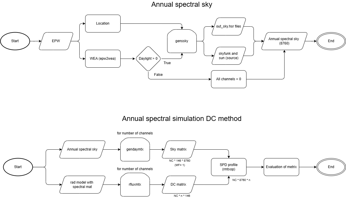
This method requires a command similar to gendaymtx to extract all annual data (or selected hours) from the EPW file, compute their spectral values, and return them as a three-dimensional matrix consisting of time, sky patches, and spectral data. Marshal Maskarenj has done something similar with EPW2AnnualSpectra, which you can find here (although I couldn’t find the source code for the executable and don’t know the exact method used). This process takes about 20 minutes per EPW file.
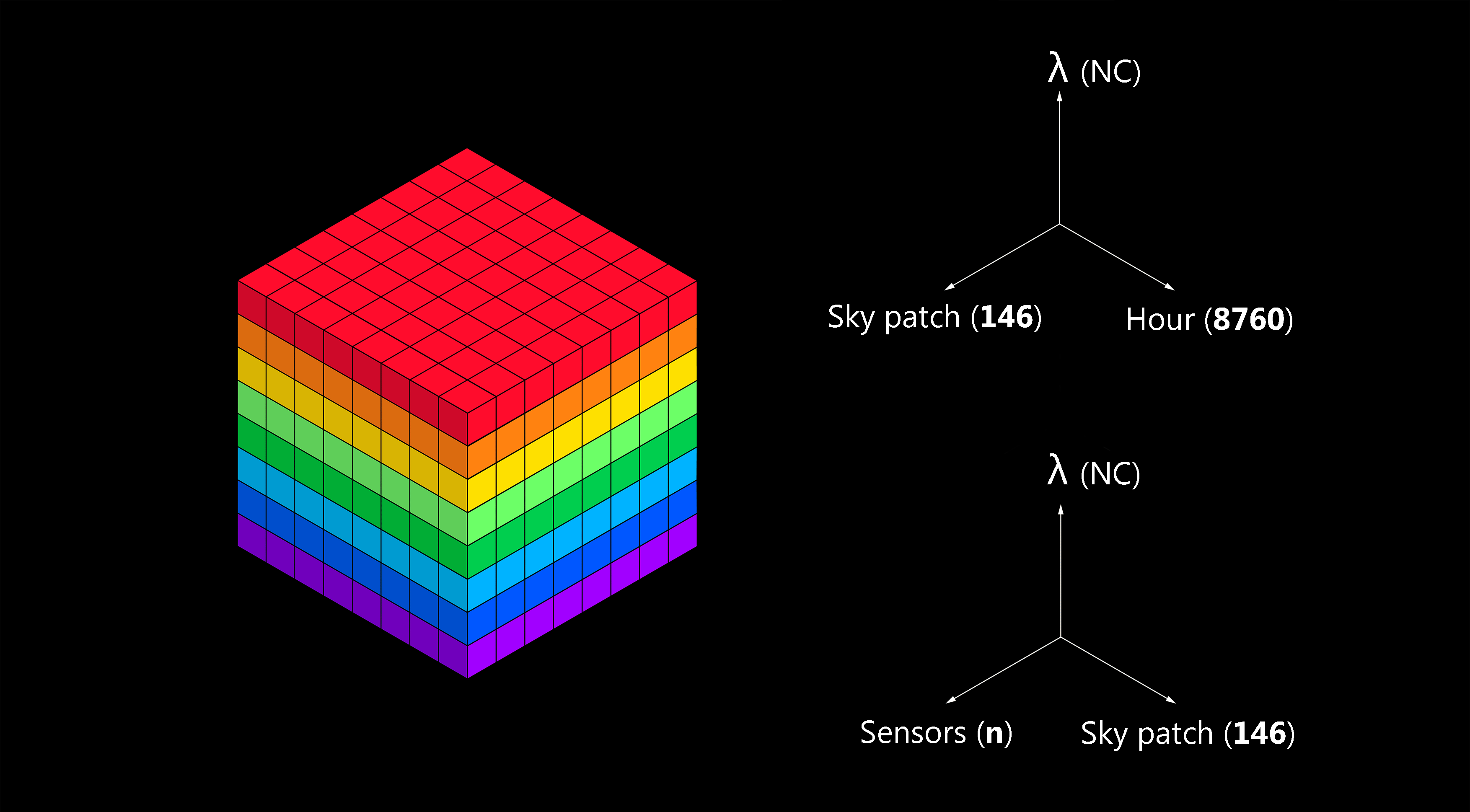
Afterward, due to variations in material reflectance and transmittance, we need to generate a DC matrix for each spectral channel (another 3D matrix). Finally, these matrices are multiplied together in sequence, resulting in a 3D matrix of sensors, time, and spectrum. By applying relevant response curves, such as the ipRGC cell sensitivity curve, we can obtain the final values.
Can we add these capabilities to commands, or do we need something completely new?
I also had a few requests:
- The output of the rtrace command seems to go from 780 to 380. Can you change the output direction from 380 to 780? In the pyradiance library, the output is also in string format, and it would be better if it could be converted to a list.
- The rtpict command does not work on Windows when spectral settings are enabled. It returns an empty hsr file, while the same python code works correctly in the Linux.
Thanks in advance