From Sarith Subramaniam publication, N-phase matrix-based methods use the high-level function rfluxmtx. That said, in Wendelin Sprenger’s PhD thesis, a distinct implementation is made with a similar objective.
From what I have been able to understand, for rfluxmtx, the transfer functions for each sky patch are made relative to the skyglow generated from a Tregenza or Reinhart distribution for the most common discretizations. In this formalism the inter-reflections are attributed to the “arrival sky patch” so that there is no more information about the angle of incidence for example at the interface with glass.
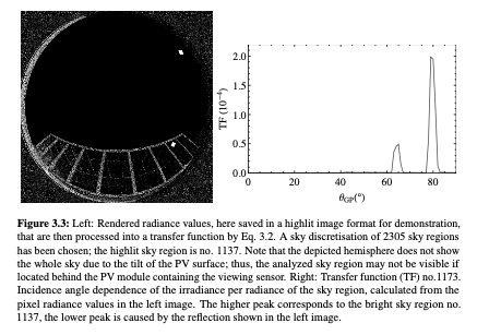
In Wendelin Sprenger’s thesis, these transfer functions are made in terms of angle of incidence so that it is possible to preserve the origin of the first bounce (see the two attached figures). Is it possible to propose a similar approach? If so, what would be the approach? Is this compatible with the gendaymtx function?
I would like to proceed as follows in order to be able to integrate complex optical structures at the level of the virtual sensor point. As a result, the geometry of the system is simplified. Also the processing is accelerated by using python scripts in post-process.
What is the exact input and output you are looking for, that got you interested in rfluxmtx, specifically? What are you trying to compute?
It is of course possible to create rays according to whatever distribution you like and send them through rtrace to determine contribution values with the -oW or -oV option. This is how rcontrib (called by rfluxmtx) was originally done. The directions can then be converted to bin numbers if you want to use them as part of an annual simulation with gendaymtx and dctimestep, etc.
My application concerns photovoltaics modules for which the number of sensors is quite large, between 50k and 100k (to give an order of magnitude) with parts in motion.
Compared to the use of Rtrace, this is justified by a desire to separate geometry and optical properties from temporal dependence of the sky (with a lower impact on results, ground is also time-varying).
At it currently stands, the use of rfluxmtx makes it possible to carry out up-to simulation at a 1 minute basis on an annual scale for plane of array solar irradiance.
With the daylight coefficient approach, the output of RADIANCE are in one side the .mtx file and on the other side the .sky file. The post-process in Python replace the internal usage of dctimestep.
I don’t have reach the level of understanding of rcontrib based on the lesson.
The continuation of this approach would be to evaluate under which conditions it is possible to separate optical properties from the geometry.
Also I would like to add a wavelength specific dimension to such simulation that why I want to remove glass layers on either side of photovoltaic modules.
That said ideally, the spectral part is reduce to the ground property (as a first approximation). Other elements of the scene are treated as neutral plastic. This allow to try an alternative to the line by line three channel simulation (N*RGB simulations) with varying optical properties.
In doing so, a post-process such as the one proposed in Windelin Sprenger’s PhD thesis allow to use transfer function matrix with an optical model that replicate the behavior of a multi-layer stack of textured materials as a function of wavelength and angle of incidence.
The good news is that the latest alpha version of Radiance now supports multi-band (i.e., hyperspectral) rendering, so you are no longer limited to 3 channels. The maximum defined by the MAXCSAMP macro at compile-time defaults to 24. You will need to get the installers for the HEAD from this link. An overview of these additions is in this PowerPoint presentation.
Regarding rcontrib, there is of course a man page, which you can use as a guide to understanding the command run by rfluxmtx. You can see this command by adding the “rfluxmtx -v” option.
Depending on how you use rfluxmtx, the creation of this rcontrib command may be all that it does. It would help me understand your process if you shared your current Radiance commands, at least the main one(s).
I’m hoping that you can use rcontrib directly, intercepting the ray directions and other information you need rather than trying to get them out of rfluxmtx.
Thank you for your reply.
The multi-band approach greatly simplifies workflow for spectral simulation if having a spectral sky model. Based on slide 15 does it mean that rfluxmtx that encapsulate rcontrib can be set with 24 spectral bands therefore the number of components NCOMP in the mtx files will be changed accordingly ?
In current command terms, the sequence is as follows:
For the irradiance time series for a neutral color simulation a dot produce in python is used.
From this implementation, front and rear glass layers should be included into the created material.rad file and in the path to geometry rad files. Otherwise by following the same approach as proposed in Wendelin Sprenger’s thesis, a post-treatment of glass layer will attenuate drastically most of reflected irradiance as with this convention, contribution are accounted based on the angle of incidence between sky patch azimuth and elevation and PV module azimuth and elevation that exceed 90° for most of the reflected component.
Yes, you should be able to use rfluxmtx with options “-cs 24” and if you like, alter the wavelength sampling range using the “-cw min_nm max_nm” option. This will generate 24 components rather than 3 out of rcontrib.
Given that you are using the -I+ option of rfluxmtx, you cannot get the actual ray directions used in sampling. If you want those, you will need to create your own ray generator using vwrays based on your sample point positions and orientations. If you have only one, this is straightforward. What is the input to rfluxmtx stdin in your case?
This is a very interesting approach, it is possible to see an application spectral band by spectral band instead of line by line which can speed up calculations for solar applications for example. This on a spectral domain subdivided not necessarily in a regular way.
The rfluxmtx stdin is a sensor points file with multiple points with position and orientation for each line. Does the use of the vwrays function follow the methods proposed in Andy McNeil’s tutorials on the Three-Phase Method?
Unfortunately, we don’t support unevenly spaced spectral samples, though I admit equal nm steps doesn’t make sense in the infrared.
The use of vwrays here is different inasmuch as we are just trying to sample the hemisphere. I’m not even sure it’s the best way, but it’s probably the simplest. Even so, the command is going to look strange and unpleasant. I am assuming you are on Unix. If you’re using Windows, you’ll need to replace the single-quotes with double-quotes and save and execute the commands in a batch file rather than passing the output of the first rcalc to sh:
The first command generates a 36 MB file with all of your ray samples for 12 sample positions.
The “rcontrib -c 127449” command corresponds to the number of rays per hemispherical sampling, which it will average together to give your result for each desired irradiance value. The final “getinfo -c rcalc” command adjusts each value for the fact that some of the rays from vwrays are zero-vectors, since they are outside the projected hemisphere circle.
I haven’t tested this, and it may well contain some bug or something I haven’t thought out.
I thank you for this script, which is quite complex at first glance, and for the description you give of it! I will make the link with the manpage documentation for a better understanding of the different fields.
On spectral sampling perhaps it is possible to see a hack in which equal steps in wavelength can represent variations of spectral profiles that are unevenly spaced. That said, in solar application, the use of unevenly distributed bands is common (for example Kato-bands between 250 and 4600 nm) and it turn out that post-process is used to recover wavelength specific steps.
Yes, if you are just doing a per-channel calculation and not using any of the Radiance tools to go to/from RGB or XYZ tristimulus, then it doesn’t matter if you remap the spectral bands. Of course, it makes the most sense to have even steps in frequency rather than wavelength, but that’s not standard practice for the visible range.